Lane Tracking via Computer Vision

As part of the first term of my Udacity Self-Driving Car program many topics relating to computer vision and how they integrate into driving a car were though, involving many projects that may be encountered in real-life attempts at programming an autonomous car.

Here I will walk through the steps I used and the techniques involved.

Calibrating and Transforming Perspective

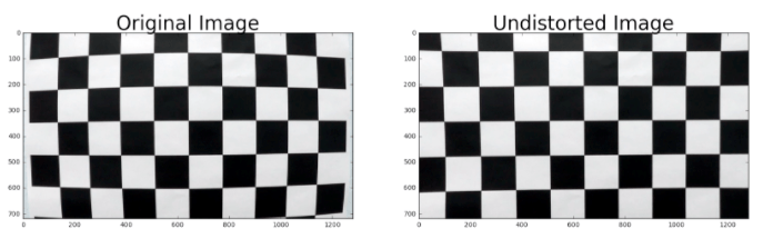
The lens of every came increases a slight portion of distortion within the images it captures, especially around the corners. Using a printed chessboard image and then tracking the corners with a function from OpenCV, the image can be transformed slightly to straighten out the lines, and then apply that transformation to subsequent images of the camera. Below is an example of image un-distortion:

def toCalibrate(img,nx,ny):
    objpoints = []
    imgpoints = []
    objp = np.zeros((nx*ny, 3), np.float32)
    objp[:,:2] = np.mgrid[0:nx,0:ny].T.reshape(-1,2) # x,y coordinates
    
    # Find chessboard corners
    ret, corners= cv2.findChessboardCorners(img, (nx,ny), None)

    # If found, draw corners
    if ret == True:
        # Draw and display the corners
        cv2.drawChessboardCorners(img, (nx, ny), corners, ret)
        imgpoints.append(corners)
        objpoints.append(objp)
        plt.suptitle('Original', fontsize=14, fontweight='bold')
        plt.imshow(img)
        plt.show()

        global mtx
        global dist
        global rvecs
        global tvecs
        global undist
        ret, mtx, dist, rvecs, tvecs = cv2.calibrateCamera(objpoints, imgpoints, toGray(img).shape[::-1], None, None)
        undist = cv2.undistort(img, mtx, dist, None, mtx)
        
        plt.suptitle('Undistorted', fontsize=14, fontweight='bold')
        plt.imshow(undist)
        plt.show()
    if ret == False:
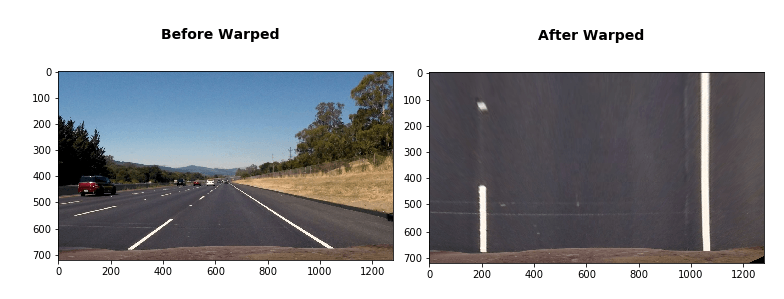
        print('Did not find any corners')

Next I need to transform the image from having a driver POV to a birds eye POV. This can be accomplished with the OpenCV function warpPerspective.

def toWarp(img,src,dst):     
    # Grab the image shape
    if len(np.shape(img)) > 2:
        img_size = (toGray(img).shape[1], toGray(img).shape[0])
    else:
        img_size = (img.shape[1], img.shape[0])
    

    #im2 = img.reshape(img.shape[0], img.shape[1])
    plt.suptitle('Before Warped', fontsize=14, fontweight='bold')
    plt.imshow(img)
    plt.show()
    #print(np.shape(gray))
    # Given src and dst points, calculate the perspective transform matrix
    M = cv2.getPerspectiveTransform(src, dst)
    # Warp the image using OpenCV warpPerspective()
    warped = cv2.warpPerspective(img, M, img_size)
    plt.suptitle('After Warped', fontsize=14, fontweight='bold')
    plt.imshow(warped)
    plt.show()
    return warped, M

Binary Transformation for explicit lane identification

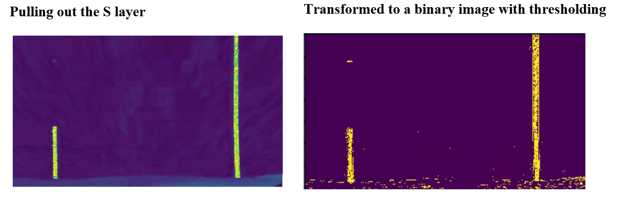
I performed a transformation of color channels to HLS and then pulled out the S layer as it seemed to perform the best in making the lane line stand out. Then using gradient thresholds to generate a binary image (values are either 0 or 255). The threshold values I used were 10 and 100. Below is an example of my output for this step.

# for a given sobel kernel size and threshold values
def toMagSobel(img, sobel_kernel=3, mag_thresh=(0, 255)):
    # Convert to grayscale
    if len(np.shape(img)) > 2:
        gray = cv2.cvtColor(img, cv2.COLOR_RGB2GRAY)
    else:
        gray = img
    # Take both Sobel x and y gradients
    sobelx = cv2.Sobel(gray, cv2.CV_64F, 1, 0, ksize=sobel_kernel)
    sobely = cv2.Sobel(gray, cv2.CV_64F, 0, 1, ksize=sobel_kernel)
    # Calculate the gradient magnitude
    gradmag = np.sqrt(sobelx**2 + sobely**2)
    # Rescale to 8 bit
    scale_factor = np.max(gradmag)/255 
    gradmag = (gradmag/scale_factor).astype(np.uint8) 
    # Create a binary image of ones where threshold is met, zeros otherwise
    binary_output = np.zeros_like(gradmag)
    binary_output[(gradmag >= mag_thresh[0]) & (gradmag <= mag_thresh[1])] = 1

    plt.suptitle('After Binary Mag Sobel', fontsize=14, fontweight='bold')
    plt.imshow(binary_output)
    plt.show()
    # Return the binary image
    return binary_output

Plot a Histogram of Pixel Values

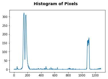
Now if we plot a histogram of the pixel values on the X-axis, it starts to really stand out where the lanes reside in the image.

plt.suptitle('After Sobel Binary', fontsize=14, fontweight='bold')
plt.imshow(step2)
plt.show()

histogram = np.sum(step2[step2.shape[0]//2:,:], axis=0)
plt.suptitle('Histogram of Pixels', fontsize=14, fontweight='bold')
plt.plot(histogram)
plt.show()

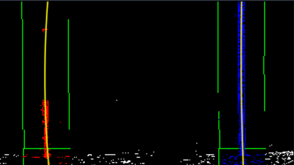
Sliding Window Detection

Breaking up the image height-wise into a series of sliding windows I can continually find the pixel locations and begin to mark the lane locations. In the below image you can see the result of this effort. Though there were some issues drawing the window rectangles, it performed well enough in practice. It uses a total of 9 windows on each lane to then track midpoint concentration of pixels, to best fit the lane line.

def regressionLanesTracker(src):
    
    binary_warped = src
    # Assuming you have created a warped binary image called "binary_warped"
    # Take a histogram of the bottom half of the image
    histogram = np.sum(binary_warped[int(binary_warped.shape[0]/2):,:], axis=0)
    # Create an output image to draw on and  visualize the result
    out_img = np.dstack((binary_warped, binary_warped, binary_warped))*255
    # Find the peak of the left and right halves of the histogram
    # These will be the starting point for the left and right lines
    midpoint = np.int_(histogram.shape[0]/2)
    leftx_base = np.argmax(histogram[:midpoint])
    rightx_base = np.argmax(histogram[midpoint:]) + midpoint

    # Choose the number of sliding windows
    nwindows = 9
    # Set height of windows
    window_height = np.int_(binary_warped.shape[0]/nwindows)
    # Identify the x and y positions of all nonzero pixels in the image
    nonzero = binary_warped.nonzero()
    nonzeroy = np.array(nonzero[0])
    nonzerox = np.array(nonzero[1])
    # Current positions to be updated for each window
    leftx_current = leftx_base
    rightx_current = rightx_base
    # Set the width of the windows +/- margin
    margin = 100
    # Set minimum number of pixels found to recenter window
    minpix = 50
    # Create empty lists to receive left and right lane pixel indices
    left_lane_inds = []
    right_lane_inds = []

    # Step through the windows one by one
    for window in range(nwindows):
        # Identify window boundaries in x and y (and right and left)
        win_y_low = binary_warped.shape[0] - (window+1)*window_height
        win_y_high = binary_warped.shape[0] - window*window_height
        win_xleft_low = leftx_current - margin
        win_xleft_high = leftx_current + margin
        win_xright_low = rightx_current - margin
        win_xright_high = rightx_current + margin
        # Draw the windows on the visualization image
        cv2.rectangle(out_img,(win_xleft_low,win_y_low),(win_xleft_high,win_y_high),(0,255,0), 2) 
        cv2.rectangle(out_img,(win_xright_low,win_y_low),(win_xright_high,win_y_high),(0,255,0), 2) 
        # Identify the nonzero pixels in x and y within the window
        good_left_inds = ((nonzeroy >= win_y_low) & (nonzeroy < win_y_high) & (nonzerox >= win_xleft_low) & (nonzerox < win_xleft_high)).nonzero()[0]
        good_right_inds = ((nonzeroy >= win_y_low) & (nonzeroy < win_y_high) & (nonzerox >= win_xright_low) & (nonzerox < win_xright_high)).nonzero()[0]
        # Append these indices to the lists
        left_lane_inds.append(good_left_inds)
        right_lane_inds.append(good_right_inds)
        # If you found > minpix pixels, recenter next window on their mean position
        if len(good_left_inds) > minpix:
            leftx_current = np.int_(np.mean(nonzerox[good_left_inds]))
        if len(good_right_inds) > minpix:        
            rightx_current = np.int_(np.mean(nonzerox[good_right_inds]))

    # Concatenate the arrays of indices
    left_lane_inds = np.concatenate(left_lane_inds)
    right_lane_inds = np.concatenate(right_lane_inds)

    # Extract left and right line pixel positions
    leftx = nonzerox[left_lane_inds]
    lefty = nonzeroy[left_lane_inds] 
    rightx = nonzerox[right_lane_inds]
    righty = nonzeroy[right_lane_inds] 

    # Fit a second order polynomial to each
    left_fit = np.polyfit(lefty, leftx, 2)
    right_fit = np.polyfit(righty, rightx, 2)


    # Generate x and y values for plotting
    ploty = np.linspace(0, binary_warped.shape[0]-1, binary_warped.shape[0] )
    left_fitx = left_fit[0]*ploty**2 + left_fit[1]*ploty + left_fit[2]
    right_fitx = right_fit[0]*ploty**2 + right_fit[1]*ploty + right_fit[2]

    # Plot it!
    out_img[nonzeroy[left_lane_inds], nonzerox[left_lane_inds]] = [255, 0, 0]
    out_img[nonzeroy[right_lane_inds], nonzerox[right_lane_inds]] = [0, 0, 255]
    plt.imshow(out_img)
    plt.plot(left_fitx, ploty, color='yellow')
    plt.plot(right_fitx, ploty, color='yellow')
    plt.xlim(0, 1280)
    plt.ylim(720, 0)
    plt.show()

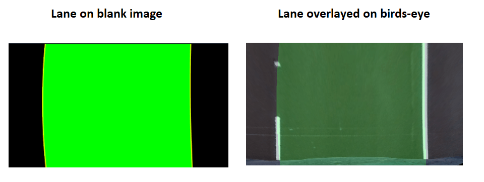
Overlay a Polygon to Fill Lanes

Once I have these lines digital lines fitted over the image of lane lines, I can use another OpenCV function to fill in a polygon and ‘draw’ a virtual lane into the birds-eye image. This function, fillPoly creates a basic polygon on a blank image, then I can use the addWeighted function to overlay it (with transparency) on to the original lane image, by first placing it on birds-eye then warping back to original.

  """
  Add polygon and Overlay and Warp
  """
def polygonOverlay(src):
  
  binary_warped = src
  # Create an image to draw the lines on
  warp_zero = np.zeros_like(binary_warped).astype(np.uint8)
  color_warp = np.dstack((warp_zero, warp_zero, warp_zero))

  # Recast the x and y points into usable format for cv2.fillPoly()
  pts_left = np.array([np.transpose(np.vstack([left_fitx, ploty]))])
  pts_right = np.array([np.flipud(np.transpose(np.vstack([right_fitx, ploty])))])
  pts = np.hstack((pts_left, pts_right))

  # Draw the lane onto the blank image
  cv2.fillPoly(color_warp, np.int_([pts]), (0,255, 0))
  plt.imshow(color_warp)
  plt.plot(left_fitx, ploty, color='yellow')
  plt.plot(right_fitx, ploty, color='yellow')
  plt.suptitle('lanes', fontsize=14, fontweight='bold')
  plt.show()
  #toWarp(fig,src=src,dst=dst)

  # Overlay polygon on birdseye
  step00 = step0.copy()
  alpha = 0.2
  temp = cv2.addWeighted(color_warp, alpha, step00, 1 - alpha,0, step00)
  plt.imshow(temp)
  plt.suptitle('lanes birdeye', fontsize=14, fontweight='bold')
  plt.show()

  # Un-un-warp function
  def unwarp(warped, M):
      img = warped
      img_size = (img.shape[1], img.shape[0])
      return cv2.warpPerspective(warped, M, img_size, 
                                 flags=cv2.WARP_INVERSE_MAP)


  # Present basic transformation of polygon
  tt = unwarp(color_warp, M)
  plt.imshow(tt)
  plt.show()

  # Create copy (so addWeighted does not stack)
  tt_copy = tt.copy()

  # Overlay the image
  alpha = .3
  temp = cv2.addWeighted(tt_copy, .3, test_images[6],1,0)
  plt.imshow(cv2.cvtColor(temp, cv2.COLOR_BGR2RGB))
  plt.show()

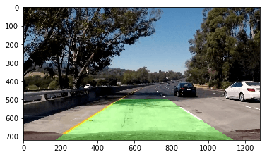
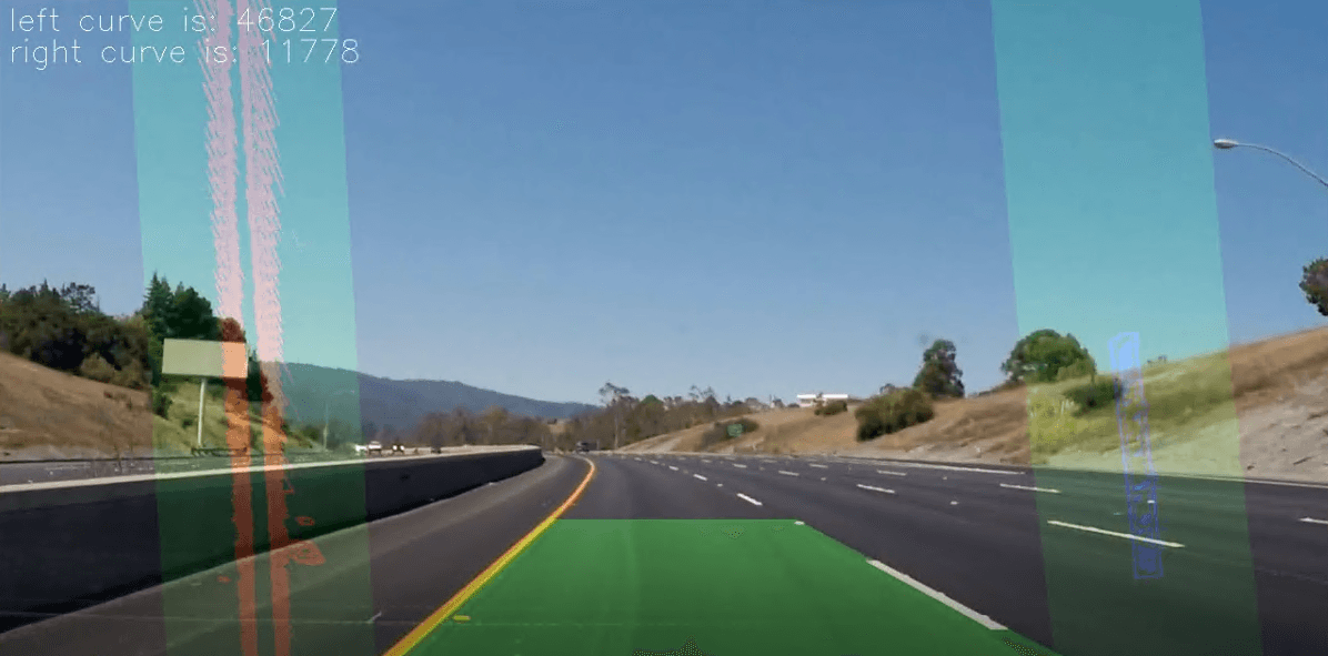
Final Steps

Now I just take the lane plotted back on to the video feed, with detected lane line curves also overlaid onto the image, along with the curves printed in the top-left corner (radius in meters).