Randomness in all its wonderful forms!
Over the years I have fallen in love with the ideas of prediction, models, and the tailwind of computer analytics that subsequently brought them all together. It’s such a fascinating time to be an observer trying my best to keep up with the steady flow of papers and talks, and the ever increasing amount of open-source code that is becoming the norm for everything from academia to the tech giants of Facebook and Google.
I wanted to be able to gather up all these scraps in my head and lay them back out in an attempt to help both me and anyone else that may come by and graze. Most of these will focus on the general area of modeling and statistics from the frame of modern machine learning, so it would be best to go ahead and explain the foundations of randomness.
Random Walks of 1000 Steps

Heads up: this is snippet-style code from 2017 that stitches a few pieces of a larger notebook together. It references x and an init callable defined elsewhere, so it won't run end-to-end as shown — treat it as a sketch of the animation structure, not a copy-pasteable script.
"""
Video animation of stock ticker charts to represent randomness

By: David Rose
Date : 10/9/2017
"""
import numpy as np
import matplotlib.pyplot as plt
import matplotlib.animation as animation
import random

from itertools import cycle
import random


# How many total lines to model (frames in the video)
lineCount = 1000

# Length of travel (total steps)
steps = 2000


# First set up the figure, the axis, and the plot element we want to animate
fig = plt.figure()
#ax = plt.axes(xlim=(-20, 20), ylim=(-20, 20))
xMin = 0
xMax = x[:,0].max()
yMin = x[:,1].min() * 1.8
yMax = x[:,1].max() * 1.8
plt.axis('equal')
#plt.title('50 random chart movements, static range (-5,5)')
ax = plt.axes(xlim=(0,steps), ylim=(-500,500),
              title=str(lineCount) + ' random chart movements, static range (-5,5)')

# Create list of various colors to cycle through for each line below
#cycol = cycle('RGBA')

def build_tickers(lineCount=3, steps=steps):
    x = np.zeros((steps,2))

    for i in range(0,len(x) - 1):
        for ii in range(0,len(x[i])):
            if ii == 0:
                # For x-value
                # Iterate 0,1,2,...
                x[i + 1][ii] = x[i][ii] + 1
            else:
                # For y-value
                # go a random direction

                n = random.randrange(-5,6,1)
                x[i + 1][ii] = x[i][ii] + n

    line, = plt.plot([], [], lw=1)
    line.set_data([], [])
    line.set_data(x[0:i,0],x[0:i,1])
    return line,


anim = animation.FuncAnimation(fig, build_tickers, init_func=init, frames=lineCount,
                               interval=2, blit=True)
anim.save('ticker_animation_test.mp4', fps=20,dpi=400, bitrate=-1,
          extra_args=['-vcodec', 'libx264'])

plt.show()
Randomness: the lack of pattern or predictability in events.
Some of the good
- It is a main component of modern cryptographic systems that power the digital age, see pseudorandom number generators.
- Simulating risk models or estimating areas using the Monte Carlo Method. (See bottom of page for example)
- Statistical inference and how it enables the ideas of surveys and the scientific method to work.
Some of the annoying
- In the age of the computer and their Deterministic method of operation, we have to ‘fake’ randomness using external sources or algorithms that can be studied > modeled > predicted. This is the method a Russian hacker used to bilk casinos out of millions of dollars.
- Due to interactions going all the way down to the quantum level, many systems can not be modeled past a certain preciseness due to ideas of Chaos and divergence of systems over time. At the most technical level they may actually be deterministic, but pragmatically not in the ways we work with them.
- In relation to above, entire fields are dedicated to these ideas such as dynamical systems and stochastic processes that underly them, in which something may be truly non-deterministic.
Modeling Random Motion in Nature
Below is a quick animation I put together with the magic of Python and MatPlotLib (annoyingly I can’t embed H.264 via HTML5 here, had to convert to GIF)
Random Travel in a 2D plane (Wiener Process)
Github code below:
"""
A simple example of an animated Brownian motion plot

By: David Rose
Date : 10/9/2017
"""
import numpy as np
import matplotlib.pyplot as plt
import matplotlib.animation as animation

# Length of array (or how long motion is modeled)
motionLength = 1000

x = np.zeros((motionLength,2))
for i in range(0,len(x) - 1):

    for ii in range(0,len(x[i])):
        n = random.choice([1,0,-1])
        x[i + 1][ii] = x[i][ii] + n

# First set up the figure, the axis, and the plot element we want to animate
fig = plt.figure()
#ax = plt.axes(xlim=(-20, 20), ylim=(-20, 20))
xyMin = x.min() * 1.2
xyMax = x.max() * 1.2
plt.axis('equal')
ax = plt.axes(xlim=(xyMin,xyMax), ylim=(xyMin,xyMax))

line, = plt.plot([], [], lw=2)

# initialization function: plot the background of each frame
def init():
    line.set_data([], [])
    return line,

def iterr(i):
    line.set_data(x[0:i,0],x[0:i,1])
    return line,


anim = animation.FuncAnimation(fig, iterr, init_func=init, frames=motionLength,
                               interval=100, blit=True)

anim.save('test_animation_2.mp4', fps=120, bitrate=-1,
          extra_args=['-vcodec', 'libx264'])

plt.show()
The Wiener Process, or Brownian Motion
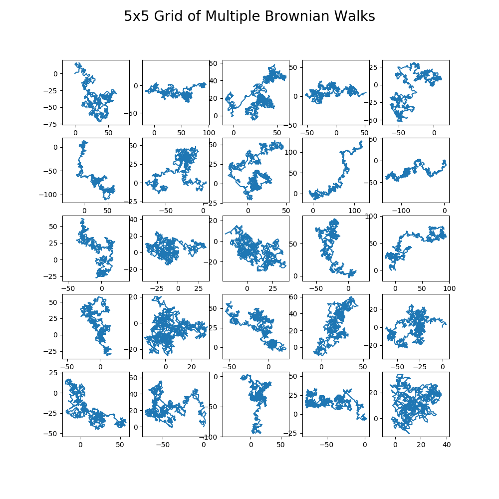
As above and below, these motions are all related to the same idea of a stochastic motion over time. The grid blow contains 25 simulations of random 2D motion to give an idea of the varying types of outcomes. As the stocks charts simulated at the top and the animation above as well illustrate, these are discrete approximations of a Wiener process. Strictly, a Wiener process is the continuous-time limit with Gaussian increments; what I'm plotting here is the integer-step random walk that converges to it. Either way, the shape shows up all over: control theory, probability, quantum mechanics, finance, and more.
Each plot below contains 1000 steps starting at 0,0 and going any direction from there. It’s interesting so see how different these can end up. When looking at a single image it may seem evident there are some clear patterns taking hold, which dissolve with each subsequent image.
Now relate this back to events someone may observe in day to day life and you can see why people may begin to see patterns where they don’t exist.
Github code below:
"""
Plot out grid of 5x5 brownian motion 2D plots
By: David Rose
Date : 10/9/2017
"""
import matplotlib.pyplot as plt
import numpy as np
import pandas as pd
import random
def brownian_model_plot(length):
# Length of array (or how long motion is modeled)
X = np.zeros((length,2))
for i in range(0,len(X) - 1):
for ii in range(0,len(X[i])):
direction = random.choice([1,0,-1,-2,2])
X[i + 1][ii] = X[i][ii] + direction
x = X[:,0]
y = X[:,1]
return x,y
fig, ax = plt.subplots(nrows=5, ncols=5, figsize=(10,10))
for row in ax:
for col in row:
x,y = brownian_model_plot(1000)
col.plot(x,y)
col.axis('equal')
plt.suptitle('5x5 Grid of Multiple Brownian Walks', fontsize=20)
plt.savefig('Brownian_Model_grid.png', dpi=100)
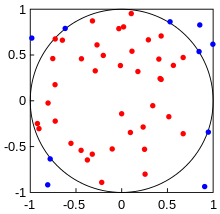
plt.show()Monte Carlo Estimation of Area
When attempting to find the area of any 2D or 3D shape you may realize there is no obvious analytical solution, unless you know the function that created it. One method that is quite simple with a computer is to simply brute force it.

Monte Carlo methods, named after the casino in gambling mecca Monaco, came about when Stanislaw Ulam looked to model the random processes that were the foundation of many gambling style games, such as roulette, dice, and slot machines. He initially theorized some of this work while performing nuclear research at Los Alamos in the late 1940’s, it was soon picked up by John von Neumann who programmed some of this into a computer to perform some calculations.
This was already possible to envisage with the beginning of the new era of fast computers, and I immediately thought of problems of neutron diffusion and other questions of mathematical physics, … Later [in 1946], I described the idea to John von Neumann, and we began to plan actual calculations.[13] — Stanislaw Ulam
Steps involved:
* Place image in a square grid
* Throw down a lot of random points
* Measure ratio of points within to overall amount
* Multiply by area of rectangle
Here is an animated plot I created that iterates through 2000 steps of random points in the box, and continually re-calculates the estimates area of the circle:
(Correct area is ~3.14)
GitHub code below:
"""
Video animation of Monte Carlo estimation of a circle's area.
The function (x**2 + y**2 + r**2) can be changed around to create other shapes of choice.

By: David Rose
Date : 10/9/2017
"""
import numpy as np
import matplotlib.pyplot as plt
import matplotlib.animation as animation
from itertools import cycle
import random


# Select dot count (more gives better accuracy!, seems to converge around ~2k normally)
dotCount = 10000

x = np.random.uniform(-1.5,1.5,dotCount)
y = np.random.uniform(-1,1,dotCount)
plotArea = 3 * 2
#print('all x is: ',x)
xx = np.linspace(-1, 1, 100)
yy = np.linspace(-1, 1, 100)
X, Y = np.meshgrid(xx,yy)
F = X**2 + Y**2 - 1

# Clear out plot memory
plt.close('all')
fig = plt.figure(2)
ax = plt.axes(xlim=(-1, 1), ylim=(-1, 1))
scat = ax.scatter([],[], s=5)

plt.contour(X,Y,F,[0])
plt.axis('equal')

def init():
    scat.set_offsets([])
    return scat

global objectArea
count = 0

def animate(i, F=F, plotArea=plotArea):
    data = np.hstack((x[:i,np.newaxis], y[:i, np.newaxis]))
    scat.set_offsets(data)

    try:
        global count
    except NameError:
        count = 0
    else:
        pass

    colors = []
    for ii in range(0,len(x) - 1):
        if x[ii]**2 + y[ii]**2 - 1 < 0:
            colors.append('blue')

        else:
            colors.append('red')
    print('-----------------',np.size(colors))
    scat.set_color(colors)

    if i < len(x):
        if x[i]**2 + y[i]**2 - 1 < 0:
            print(x[i],",",y[i], ' is in, count is now ',count)
            count = count + 1
            #scat.set_color('blue')
            #print('now count is ',count)
        else:
            print(x[i],",",y[i], ' is out')
            #scat.set_color('red')

    objectArea = plotArea * (count / (i + 1))
    areaStr = str(round(objectArea, 2))

    plt.title('Current Estimate of Circle\'s area is: ' + areaStr)

    if i == len(x):
        objectArea = plotArea * (count / len(x))
        print(objectArea)
        print(count)
        print('Monte Carlo Estimation is: ',objectArea)

    return scat

anim = animation.FuncAnimation(fig, animate, init_func=init, frames=len(x)+1,
                               interval=2, blit=False)

anim.save('monte_carlo_test.mp4', fps=20,dpi=200, bitrate=-1,
          extra_args=['-vcodec', 'libx264'])
Originally published on Medium.