Nearby Prompts, Distant Trajectories

Most people have heard of the butterfly effect. A butterfly flaps its wings in Brazil, and a month later there's a tornado in Texas. It's a great line. It's also, in pop culture, mostly vibes. People treat it as a synonym for randomness, or for cosmic bad luck, or for the vague idea that small things sometimes matter.

That's not what the butterfly effect is. The butterfly effect is a specific property of a specific kind of system: deterministic amplification of small differences. Same equations, same rules, two almost identical starting points, and the trajectories peel apart at a rate you can actually measure. There's no dice in the room. The dice aren't the point. The point is that the system does something to the starting gap that makes it grow.

That distinction is the entire reason I want to talk about it in the context of language models. A lot of people, when they see an LLM give a different answer to a slightly different prompt, shrug and say "well, it's a probabilistic model, this is temperature, seed, whatever." And some of the time they're right. But that reflex, in my experience, papers over a different phenomenon, one that doesn't depend on sampling at all, and that turns out to behave like the thing physicists call sensitive dependence on initial conditions.

What I want to do in this post is lay out the framing carefully. What chaos actually is, why it isn't randomness, why trained neural networks sit in the neighborhood of chaotic systems, what "state" even means in a language model, and why the cleanest probe of the effect I'm interested in is the most boring decoder setting you can imagine: argmax, no sampling, seed inert, temperature zero.

This is the first of two posts. This one is the lens. The next one is the experiment, where I run the lens over about 21 models and get into what moves, what doesn't, and the ways the measurement itself tries to trick you. If you want to skip ahead, the findings are in Measuring LLM Sensitivity. If you want the argument for why they matter, stay here.

What I am and am not claiming

Let me lift the obvious objections off the table first, because this is the kind of territory where people who like physics get nervous about people who like LLMs, and vice versa.

I am not claiming LLMs are chaotic in the formal sense. Classical chaos requires things LLMs don't have: an infinitely iterated map, the ability to take perturbations to zero, asymptotic time. LLMs have finite depth, finite context, and a discrete token space. You cannot, cleanly, take the limit needed for a Lyapunov exponent.

I am not claiming bigger models are more stable. I am not claiming reasoning models are more stable. I am not claiming that lower divergence is better. Stability is a property of a system, not a score. A model that outputs "the the the" forever, regardless of prompt, is extremely stable. It's also useless. We'll come back to that.

I am not claiming that sentence-embedding cosine distance is ground truth for "how much did the output change." It's a proxy. It has failure modes. I'll show you several.

What I am claiming is something narrower. At inference time, an LLM is what I'd call a hybrid sequential system. Continuous activations flowing through a stack of layers, feeding a discrete branching process at the output. Small changes in the input can do one of two things. They can move the next-token distribution a little (a bulk shift), or they can flip the argmax onto a different branch (a boundary crossing). Once a branch flips, autoregression takes over, and the rest of the generation runs on a different prefix. The system compounds.

Whether that compounding is big enough to care about depends on the model, the prompt, and the metric. That's an empirical question, and it's what the second post is about. But before the numbers, the framing has to be right, because without the framing the numbers look like noise.

Chaos isn't randomness

I want to spend some time on the physics, because the word "chaos" is doing a lot of work in this post, and I think the only way to use it honestly is to remember what it originally means.

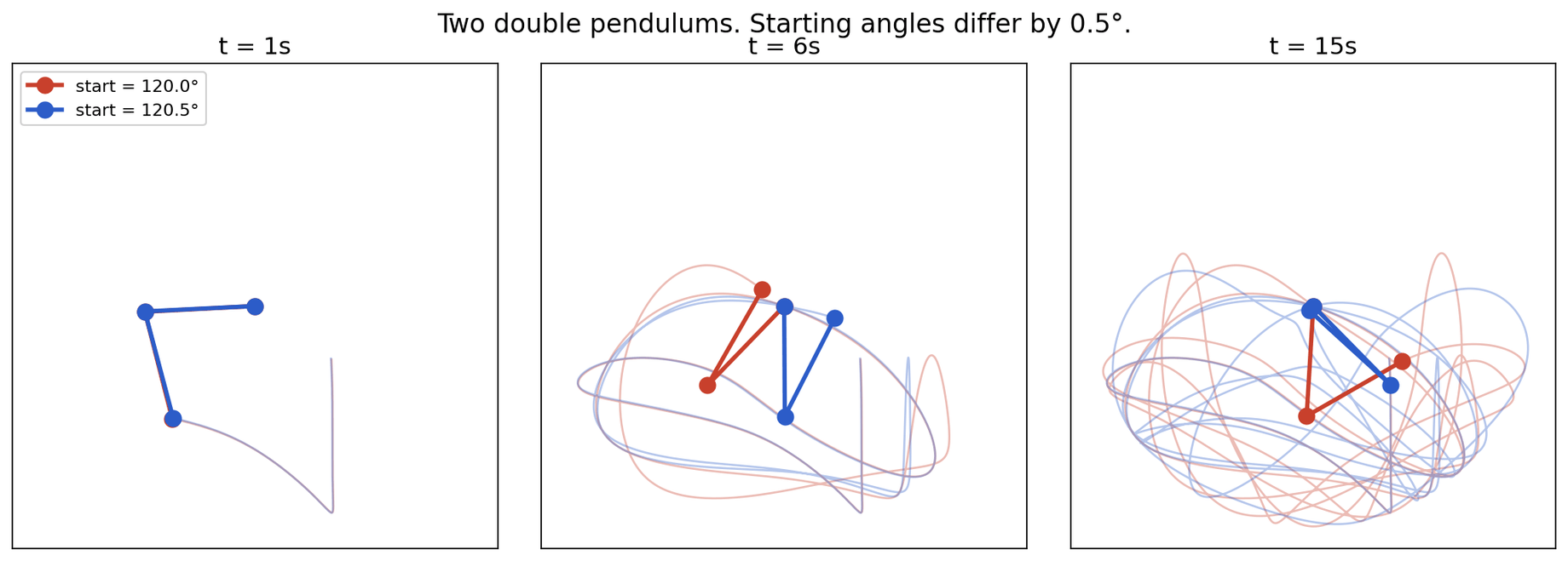
Chaos, in the technical sense, is deterministic amplification of small differences. Take two pendulums. Same mass, same length, same gravity, same initial push, except one is released at an angle that's off by half a degree. In a simple single pendulum, that half-degree difference stays small forever. The two pendulums track each other. But in a double pendulum, where the second arm is attached to the first and free to swing, that half-degree difference grows. Within a few seconds the two pendulums are in completely different places. Not because of noise. Not because of a random kick. Because the equations of motion, running deterministically, take the tiny gap you started with and stretch it.

This is not metaphor. It's mechanics. If you write down the Hamiltonian and integrate it, you can compute the rate of divergence. There's a number that quantifies it: the Lyapunov exponent, usually written as lambda. If two trajectories start a distance δ(0) apart, their separation at time t grows roughly like |δ(t)| ≈ |δ(0)| · e^(λt). If lambda is positive, the gap grows exponentially. If lambda is zero, the system is on the edge. If lambda is negative, the gap shrinks, and small differences get forgotten.

The Lyapunov exponent is the formal content of "the butterfly effect." It's a time-averaged local stretching rate. It's what lets us say something precise about how fast a weather forecast degrades, or how predictable a pool shot is after the sixth collision (answer: not very). It's also, importantly, a property of the dynamics, not a property of the initial conditions. The system either stretches or it doesn't.

The cleanest teaching example of this is the logistic map. One equation, one knob, and the whole route to chaos sitting in a single chart.

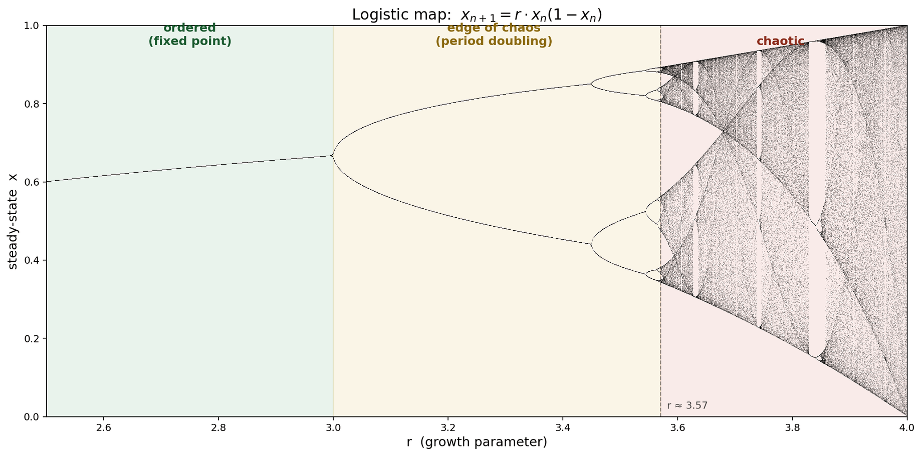
The logistic map is x_{n+1} = r · x · (1 - x). You pick a starting value for x between zero and one, pick a value for the knob r, and iterate. That's the whole system.

The chart above is a bifurcation diagram, and it is possibly the most misread image in applied math. The x-axis is r, the knob. It is not time. Each vertical slice is an independent experiment: fix r, iterate for thousands of steps, throw away the transient, plot every value the system ends up visiting. For low r the system settles on one value, so the slice is one dot. Turn r up past about 3, and the system can't hold onto a single value anymore. It starts alternating between two values forever. Period two. Turn it up more, four values. Eight. Sixteen. The splits accelerate, pile up, and by r around 3.57 the column is a smear. The system never repeats. That's chaos, visible with your eyes.

The reason this chart is a canonical piece of applied math isn't because dripping faucets are interesting, though they happen to be in this same universality class. It's because Feigenbaum showed in 1978 that a huge class of one-dimensional folding maps follows this same period-doubling route to chaos, with the same constant in front of it. Fluid onset in certain convection regimes. Some laser intensities. Some electronic oscillators. Heart arrhythmias, at some knob settings. Different systems, same bifurcation cascade. The logistic map is the harmonic oscillator of chaos: not a specific thing, but representative of a broad class.

I want to name one thing the chart is not. It is not a model of an LLM. LLMs are not a one-dimensional folding map. I am borrowing vocabulary here, not geometry. Fixed points, attractors, bifurcations, Lyapunov exponents, edge of chaos. These are the words the chart teaches, and they are the words I'm going to reach for when I describe how a small prompt change produces a big output change. The words buy nothing on their own. What buys something is the next paragraph.

Trained neural networks sit near the chaos boundary

This is the load-bearing citation chain, and it's the reason I feel okay using chaos vocabulary at all. The claim is not that I have proven LLMs are chaotic. The claim is that the family of systems LLMs belong to is already known, by the neural net signal-propagation literature, to live in a narrow band between ordered and chaotic regimes, because that's where they can be trained.

The story has three waves.

Langton, 1990, "Computation at the Edge of Chaos." Cellular automata, not neural nets. Langton showed that interesting computation, meaning the ability to propagate signals over long distances and remember things, happens in a narrow parameter band between fully ordered (everything freezes) and fully chaotic (signals decorrelate to noise). Outside that band, you can't compute. Inside it, you can.

Poole et al. 2016, Schoenholz et al. 2017. Deep feedforward networks. They show, with actual math rather than metaphor, that at random initialization, signals propagating through a deep network either shrink to zero (ordered regime, gradient vanishes) or blow up (chaotic regime, gradient explodes). Trainable networks have to be initialized near the edge between those regimes. That's not a metaphor, that's the condition for trainability. The "edge of chaos" is a specific surface in hyperparameter space (weight variance, nonlinearity gain), and if you initialize off it, learning doesn't work.

Zhang 2024 is the transformer-era reprise of the same story. Similar framing, similar conclusion, carried across to modern architectures.

I want to be careful with how I use this. The edge-of-chaos literature is about signal propagation during training in feedforward networks, not about prompt sensitivity during greedy decoding of a trained autoregressive LLM. One does not automatically imply the other. What I'd say honestly is that the two phenomena share mathematical ancestry (stretching, gradient dynamics, sensitive dependence), and the vocabulary from one is disciplined enough to be useful when discussing the other, without me claiming they're identical.

So when I say trained neural networks sit near the chaos boundary, I mean: the conditions under which deep networks are trainable overlap with the conditions the signal-propagation literature calls edge-of-chaos, and that's the vocabulary I'm going to reach for. The strong version ("LLM prompt sensitivity is literally chaos in the physicists' sense") is more than I want to defend here. The weaker version ("chaos theory supplies disciplined vocabulary for describing sensitivity in a system that discretizes stretched continuous states into branch points") is the one I'm actually using.

That's what buys me permission to use chaos vocabulary for LLMs at all. The honest question isn't "are LLMs chaotic." It's narrower: "for a given trained LLM at inference time, on this input, how much does the response function amplify a small change, and does that vary in ways we can measure?"

Is an LLM a dynamical system?

Let me run the checklist.

A dynamical system has state. LLMs have state: per-layer residual activations, logits, the prefix of tokens generated so far, the KV cache that backs attention over that prefix. That's a lot of state. Forty-eight layers, thousands of dimensions per layer, growing context. It's not small.

A dynamical system has iteration. LLMs iterate: each forward pass produces a token, the token gets appended to the prefix, the prefix conditions the next forward pass. That's autoregression. Same function, applied repeatedly, with the output of step n fed back as input to step n+1. The logistic map also has this shape. So does every other iterated map in the dynamical systems textbook.

A dynamical system is typically deterministic, at least when you want to analyze it. LLMs are deterministic under argmax decoding: do_sample=False in the HuggingFace transformers API, which picks the highest-logit token at every step. No sampling. The seed is inert. Run the same prompt through the same weights twice with argmax decode, and you get byte-identical output up to GPU kernel nondeterminism (which is tiny and not the source of the effects I'm measuring).

A dynamical system can amplify small input differences. LLMs can too, at least sometimes, and the whole second post is about measuring exactly that, carefully, across many models. Here's one preview example to give the question a concrete shape, with the understanding that it's one datapoint, not the study. OLMo-3 7B. Prompt A: "write a concise Python palindrome function." Prompt B: the exact same string, with a single trailing space after the period. Argmax decode. Same weights. Same seed. No temperature.

Prompt A gives a clean utility function with a docstring. Prompt B gives a chatty conversational preamble followed by a one-liner implementation. Two different answers from one trailing space, under deterministic decode. That's the kind of thing the rest of this work asks: how often, in which models, and under what conditions. The answer is more structured than "any byte flips the model," but it's also much less boring than "they're basically the same."

So on the checklist, an LLM at inference has state, has iteration, is deterministic, and can amplify small input changes. It fits. What the checklist doesn't tell you is the magnitude of the amplification, or whether the magnitude is the same across models, or how to measure it cleanly. That's what the rest of this work is about.

There is a catch worth naming. Classical chaos wants to take input perturbations to zero, because the math is an asymptotic statement about infinitesimal separations. Token space is discrete. The smallest perturbation in token space is one token. You can't take the limit. So anything I do here is going to be a finite-perturbation probe of a discretized system, and I will never be able to cleanly compute a classical Lyapunov exponent at the text level. I can measure response functions, and I can compare across models, but I have to be honest about what the probe is.

An interactive detour

If the stretching-rate argument above felt abstract, it might help to actually see a ripple propagate through something that sort of looks like a tiny network. This is a toy. It is not a real language model. It is not even a real neural net. It's a few rows of cells where each cell's next state depends on its current state and its neighbors, and you can click to perturb one cell and watch the disturbance spread.

The point of the toy isn't fidelity, it's intuition: the same local rule, applied everywhere, can either swallow a disturbance or amplify it, depending on the regime. Click around a bit.

What that toy is showing you isn't specific to language models. It's showing you the condition for chaos: a local rule that, iterated over state, can take a tiny perturbation and not let it dissipate. The logistic map has this property at high r. A double pendulum has it over most of its parameter space. A signal-propagation-tuned neural net has it in the regime where it's trainable. The rule has to stretch.

Temperature is a different axis

The most common pushback I've gotten when I show the OLMo trailing-space example is: "okay, but isn't that just temperature?" I want to kill this conflation right now, because it's two different phenomena, and people collapse them.

Temperature is a parameter that controls sampling. You have a fixed next-token distribution, computed by the model for a given input. Temperature T rescales the logits before the softmax: p_i ∝ exp(logit_i / T). As T goes to zero, the distribution collapses to the argmax (all mass on the max-logit token). At T = 1, you get the raw distribution. As T grows, the distribution flattens toward uniform. Temperature is how peaked or flat the distribution is, when you draw from it.

Sensitivity is a different question. Sensitivity asks: when the input changes a little, how much does the distribution itself move? Before you sample anything. You have a distribution given the original prompt, and a distribution given the perturbed prompt, and the question is the distance between those two distributions.

These are orthogonal axes. You can have zero sampling noise (temperature zero) and still see the output move a lot. You can also have high sampling noise and a rock-solid distribution. They don't have anything to do with each other, and mixing them up makes the experiment unrunnable.

Here's the 2x2 that unsticks it for me. Same prompt, temperature zero: byte-identical output. That's just determinism. Same prompt, temperature above zero: different draws, same underlying distribution. That's sampling noise, and it's boring. Different prompt, temperature above zero: different draws and different distributions. You can't tell the two effects apart. Confounded. Different prompt, temperature zero: sampling step is gone, so any movement is the response function of the model itself. The distribution moved. Clean probe.

That last cell, different prompt at temperature zero, is what the rest of this project measures. The whole experimental apparatus is built around stripping out sampling so that what's left is the model's functional response to input.

One line, because this is the pedagogical linchpin: temperature samples from a distribution. Sensitivity asks how far the distribution moved. If you only remember one thing from this post, I'd take that.

When I walk through this in talks, someone usually asks: "but what if I set T = 0.1? That's still low sampling noise, won't the result be the same?" I ran that control on OLMo-3, thirty samples per prompt, temperature 0.1, on the palindrome pair. Prompt A's samples cluster tightly. Prompt B's samples cluster tightly. The two clusters are visibly separate, and the distance between them is larger than the spread within either. Meaning: even with a little temperature, the sensitivity signal dominates the sampling noise. Two attractors, not one unlucky draw. I stopped using T > 0 as a probe after that, because it only confuses the measurement and doesn't add anything.

Meaning-preserving perturbations

There's a subtlety here that matters for how you interpret any of the results. When a prompt perturbation produces a different output, that's not necessarily the model making a mistake. A double pendulum isn't wrong when it lands somewhere different after a half-degree nudge. The physics is working as advertised. The pendulum is expressing sensitive dependence, which is a property of the system, not a bug.

Same bar for LLMs. If I ask "recommend a book like Dune" and the model says Foundation, and I ask "recommend a book like Dune " (with a trailing space) and the model says The Left Hand of Darkness, both answers are defensible recommendations to a human reader. Neither is a hallucination. The model picked a different basin of its response manifold. That's interesting to measure, but it's not a failure.

It also tells me what the right quantity to measure is. Not just "how much did the output change," but output change per unit of meaning-preserving input change. If you stick the word "NOT" in front of the prompt, of course the output moves. The meaning changed. That's the model working correctly. The interesting case is when the meaning didn't change, and the output moved anyway. That's where the chaos lens starts to pay off.

"Meaning-preserving" is fuzzy, and I want to flag that. A synonym swap isn't perfectly meaning-equivalent, a paraphrase really does shift nuance, and whether a duplicated period carries any semantic load is a question a linguist would happily argue for an hour. The perturbations I use in the second post aren't claimed to be semantically identical to the original. They're claimed to be the kind of change a human reader wouldn't flag as asking a different question. That's a softer version of meaning preservation, but it's the right one for the probe: changes that feel invisible, yet still sometimes move the output. Plus a positive control, a genuinely meaning-changing edit, as a sanity check that the model does respond to real semantic changes. It always does, massively, so the control is tight.

State, and what Li et al. actually measured

I want to stop for a minute on prior work, because I am not the first person to try to put dynamical systems vocabulary on an LLM, and there's a specific paper that did the rigorous version of this inside activation space while I was doing the broad version of it at the output-text level. The two are complementary and I want to be clear about where mine sits.

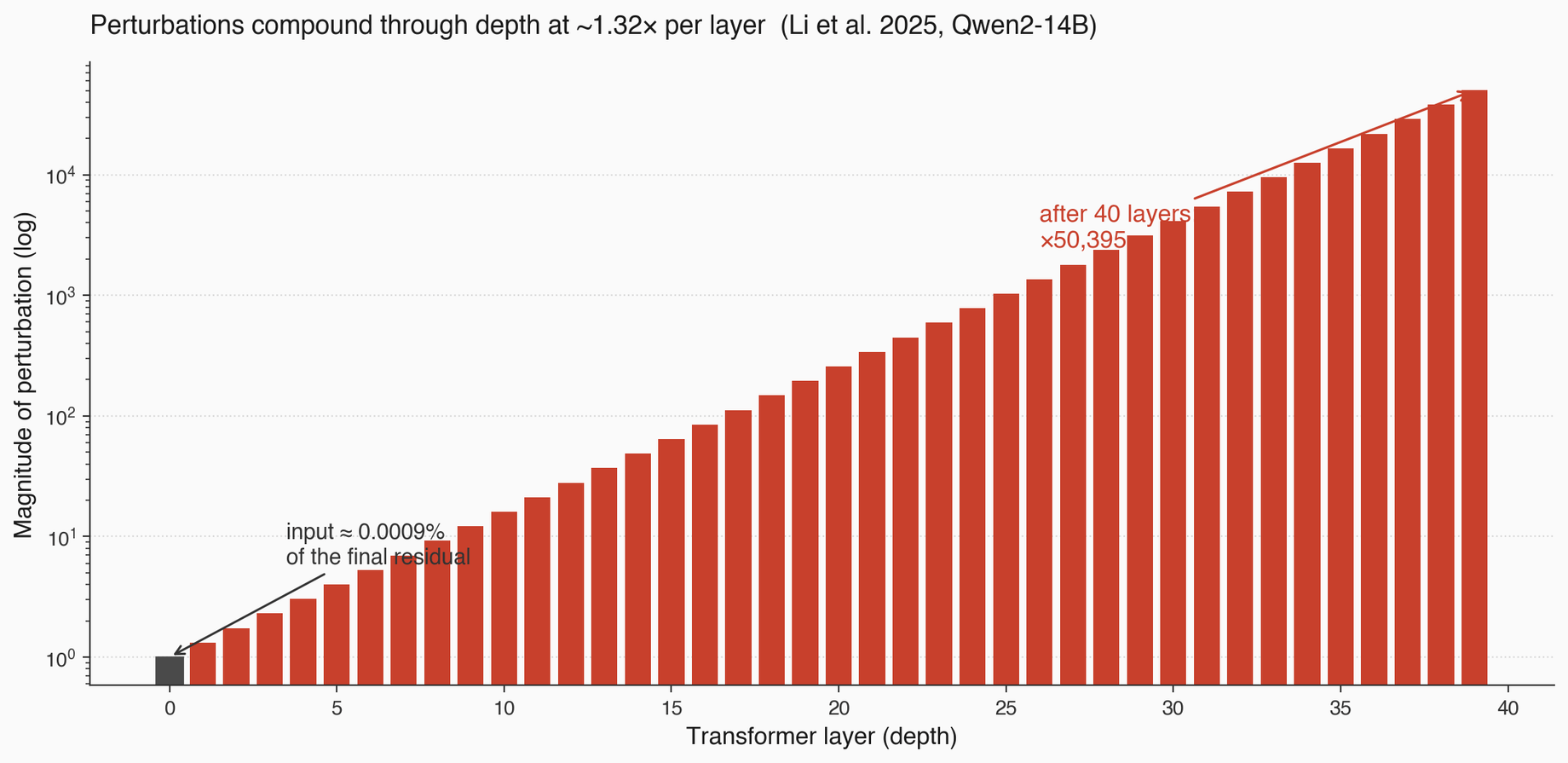
The paper is Li et al. 2025, quasi-Lyapunov analysis on Qwen2-14B. They call it quasi-Lyapunov because classical Lyapunov needs infinite iteration of a fixed map, and LLMs have finite depth. The finite-depth analog is the per-layer Jacobian norm: if I perturb the residual stream at layer n, how much does the perturbation grow by layer n+1? Average that over layers, and you get a per-layer stretching rate. Which is: the time-averaged local stretching rate, but with "time" replaced by "depth."

The number they get is about 1.32x per layer in the first ten layers. Compounded over depth, that's orders of magnitude of amplification. A tiny perturbation in the input embedding becomes a meaningful perturbation in the final residual stream.

The sharper framing, though, is their residual-stream decomposition at the final layer. MLP contributes 55.8% of the final residual. Attention contributes 44.2%. The initial input embedding contributes 0.0009%. That's chaos in one line: we perturb the 0.0009% and watch the 100% move. Almost everything in the output is transformations done inside the network. The input is a tiny seed, and the network massively amplifies it.

Here's the demo I built while I was trying to internalize this. It's a toy visualization of a perturbation propagating through a stack of "layers" with a stretching rate you can adjust. Not real activations, but the right shape.

Li et al. ran one model. They defined a token-level iterative exponent in their paper but never actually computed it, and they never compared across models. That gap, text-level across many models, is exactly where my experiments sit. I'm not doing the rigorous activation-space math they did. I'm doing the shadow at the output level, across a zoo of models, to ask which models are more sensitive and where the failure modes of the measurement lie.

Two probes of the same system, from different angles. I would never claim their math. They never claimed my breadth. It's complementary.

Also worth naming: Geshkovski et al. 2023 treat attention layers as interacting-particle dynamics, tokens as particles, attention as the interaction force. Tomihari and Karakida 2025 do a Jacobian-Lyapunov analysis specifically for self-attention. The field has been pointing at this for a while. I'm just one more data point in a longer conversation.

What the whole thing actually is

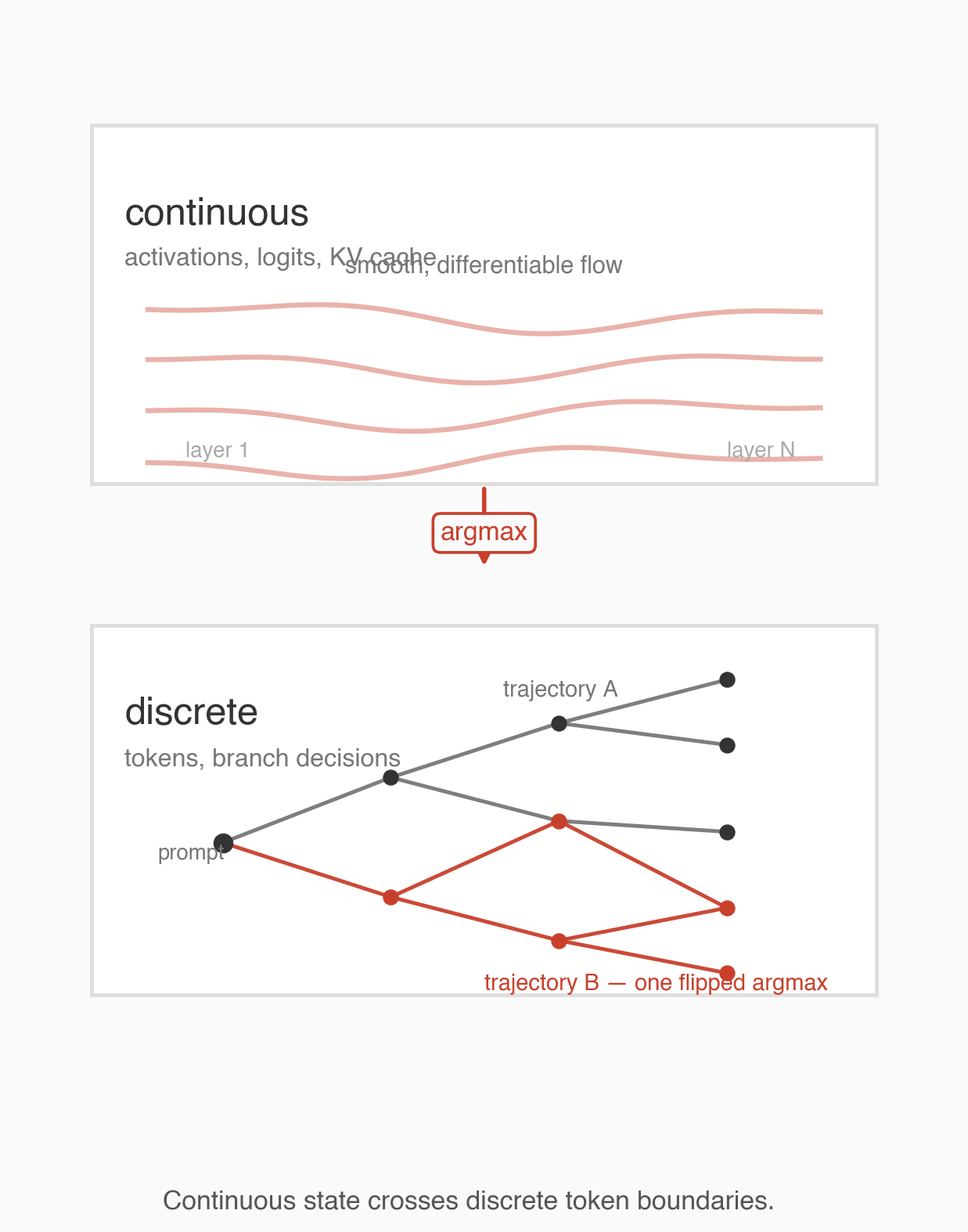
An LLM at inference time is a hybrid system. Continuous activations flowing through a stack of transformer layers, producing a next-token distribution. A discrete selection (argmax, or sampling) picks one token from that distribution. The chosen token appends to the prefix. The prefix is the input to the next forward pass. Repeat.

The continuous part stretches. Li et al. quantify the stretching at roughly 1.32x per layer in activation space for Qwen2-14B. The stretching means that a small perturbation in the input, carried through the stack, becomes a meaningful perturbation in the logits at the output.

The discrete part branches. At the top-1 selection step, a perturbation can do one of two things. If the perturbation is small relative to the margin between top-1 and top-2 logits, the argmax stays the same, and the branch is preserved. If the perturbation is large relative to the margin, the argmax flips, and the branch changes. Once a branch flips, the prefix for every subsequent forward pass is different, and the entire downstream trajectory is different.

So the stability of a generation depends on two things. One: how much the input perturbation gets amplified through the continuous stretching. Two: how many thin boundaries the generation passes through, where a small logit perturbation is enough to flip the top-1. The first is a property of the weights (Li et al.'s per-layer stretching). The second is a property of the weights and the prompt, because whether a given step sits on a low-margin boundary depends on what the model is trying to do at that step.

This is why I don't want to give you a single scalar "how chaotic is this LLM" number. The system doesn't have one. It has a stretching rate, and it has a boundary-density pattern over generation, and both of them matter. The headline from the second post is that they don't always move together, which is where the cleanest experimental dissociations come from.

What I did next, and why there's a second post

Given the lens above, the question I wanted to answer is: across a reasonable slice of publicly available models, how sensitive are they to meaning-preserving prompt perturbations? Not one model. Not in activation space. At the output-text level, where anyone can reproduce the probe, across a zoo of architectures and sizes and training recipes, with enough care that I can tell signal from measurement artifact.

I ran about 21 models, from Qwen 0.8B to Qwen 9B, Gemma, Phi-4, DeepSeek-R1, Mistral, Granite, Falcon, SmolLM, OLMo 2 and 3, plus legacy models for reference (GPT-2 XL, GPT-J, Pythia, OPT, LLaMA-1). A ladder of perturbations: identical prompt (the zero control), formatting no-ops, punctuation tweaks, synonym swaps, paraphrases, small semantic changes, and a positive control that changes meaning on purpose. Deterministic decode, do_sample=False, pinned model revisions, bf16, chat templates handled explicitly. A primary metric (sentence-embedding cosine distance) and a handful of supporting metrics (token edit distance, hidden-state distance, JS and KL on logits) because no single metric is safe alone.

What came back, I wasn't expecting most of. A heatmap of edits by model where the rows told the clearer story, not the columns. A finding that short-output stability of reasoning models is mostly a metric artifact driven by identical scaffolding preambles, and collapses when you run long. A case where a 2023 base model (LLaMA-1) turned out to be more content-stable than a 2024 reasoning model, just cleanly, in its 512-token outputs. A cleanest-in-the-panel dissociation on Phi-4 where the prompt-end distribution is effectively frozen (JS divergence of 1.4e-9, top-1 probability of 0.99999996) and yet the 512-token output diverges at 0.160, higher than GPT-2 XL. And a principled observation about the difference between stability and responsiveness that showed up in a Qwen 0.8B quantization sweep I ran almost as an afterthought.

All of that is in the second post: Measuring LLM Sensitivity: What Actually Moves the Output. The framing here is what makes those results mean something. Without it, the second post just looks like a pile of benchmarks with weird conclusions. With it, the conclusions start organizing.

One last thing before the numbers

I want to close by saying what this work is and isn't, because it's easy to over-read.

This isn't a benchmark paper. I am not proposing a new leaderboard, and I'd be uncomfortable if anyone cited specific model orderings from my results as if they were rankings. The sample sizes are small (9 to 24 prompt pairs per model cell). The cluster structure is more reliable than the within-cluster ordering. Where I give numbers, I give them because they're striking examples of principles, not because they're the final word on any model.

It's also not a proof that LLMs are chaotic. I said this at the top and I'll say it again. The honest summary is: small input perturbations produce measurable, model-dependent, reproducible output divergence under deterministic decode. That's consistent with behavior near a chaos boundary, which is independently known to be where trained neural networks live. The chaos lens is a way to organize what's happening, not a theorem I proved.

What this is, is an attempt to do the measurement honestly. To name the failure modes of the probe before anyone starts quoting numbers. To give practitioners a sharper mental model of what "this model is stable" could even mean, and why the naive version of that sentence has traps in it. To point at the questions a dynamical-systems lens suggests that benchmarks don't usually ask: what is the distance between two responses to nearby prompts, how does it scale with output length, how does it interact with reasoning scaffolds, and what's the relationship between confident logits and stable trajectories (spoiler, weaker than you'd think).

If you get nothing else from the framing post, get this: greedy LLM inference is locally stable until it isn't, and the only responsible unit of testing is the prompt neighborhood. The chaos lens is a way to organize why that's true. But the practical instruction survives even if you disagree with the framing entirely: test neighborhoods, not single prompts.

On to the experiment. Part 2: Measuring LLM Sensitivity.